Tips and tricks for using artificial speckles, both the static DM surface speckles and the dynamic ones created
using DM probes (which we call “sparkles”). The key to achieving good results is to record and reduce both the
saturated/occulted images (hereafter “sats”) and the
unsaturated/unocculted images (hereafter “unsats”) in exactly the same way.
Steps to consider when recording data with artificial speckles
You will be limited by SNR in the unsats, so make sure you take enough data to beat down the noise.
For use as a photometric and PSF reference, it is best if the sats and unsats have the same jitter so that they
have the same Strehl ratio. Since the unsats are likely taken at a higher framerate (to stay unsaturated!)
consider coadding without registration to the same exposure time as the sats.
Warning
Unsolved problem (as of June 2025): when we run the LOWFS loop to control jitter in the coronagraph, the sats will
have lower jitter than the unsats (which can’t have the fast jitter loop). This shouldn’t make a significant difference
for image registration, but for PSF photometry it could have a large effect. Below we describe an in-development procedure
to correct for this problem.
For sparkles, try to optimize amplitude (i.e. brightness) so they are both visible in unsats in a reasonable amount of time
but do not overwhelm the sats.
For sparkles with the coronagraph, consider taking unsats with the sparkles both on and off to allow subtracting the Airy
pattern and diffraction spike structure. For example, when the sparkles are at 45 degrees they land on the spikes which
are not present in a coronagraphic image, resulting in differences in the speckle background which could bias the cross-correlation.
Consider taking unsats frequently during a long observation. Due to WFS camera drifts and general alignment drifts
the PSF changes over time, as do conditions and resulting AO performance. The speckles themselves could also
change shape due to ADC problems. Anecodotally, Strehl ratio is always lowest
at the end of an observation.
The artificial speckles can be used to register images when the central star is saturated or occulted by a coronagraph.
The following recipe has been shown to give good results:
unsats
We use the unsats to establish the reference image, which has the star precisely centered on our desired
pixel (i.e. the center of rotation for ADI).
Perform a precise registration and centering of the unsats using a fit to the core of the PSF.
(see above for discussion of matching jitter). A Gaussian is probably fine
but make sure you tune the fit so it is not biased by the Airy rings, etc. An Airy pattern fit may be
more robust.
Calculate the average image. Mean combination is normally fine. A median can be used if there are hot pixels, etc.
If you were smart enough to take sparkle-off images, reduce them the same way and then subtract the resulting PSF
reference.
Radial Profile Subtraction (RPS): Subtract a radial profile from the average image. Make sure the radial profile is centered under the star.
Construct a 1/0 mask which contains only the speckles. This is to prevent the cross-correlation from being biased by
other structure in the image. The mask should be small, but be large enough to go to ~0 in the RPS images at the
edges of the mask and to account for jitter and drifts in the sat speckle locations. For the highly elongated
DM speckles this should be made out of ellipses.
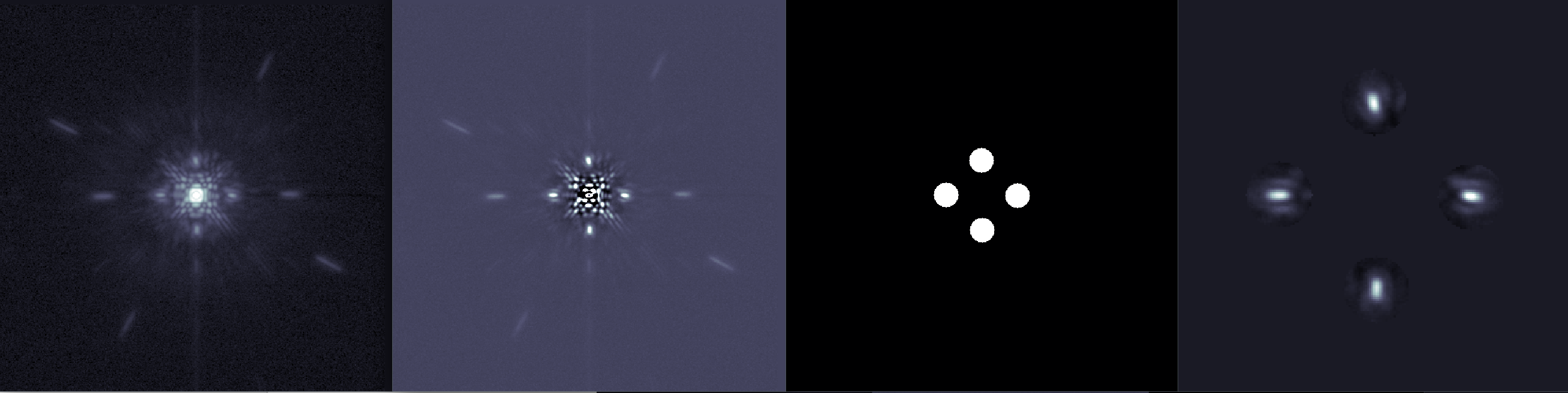
From left to right: the registered mean-combined unsat image, aligned to the center pixel;
after radial profile subtraction; the mask to isolate the “sparkles”; a zoomed-in image showing
masked sparkles. The right-most image is the reference for cross-correlation.
Construct a 2D Tukey window based on the mask, using
a low alpha so the actual speckle flux is not attenuated. This is needed to deal with the discontinuity caused by
normalization (discussed below).
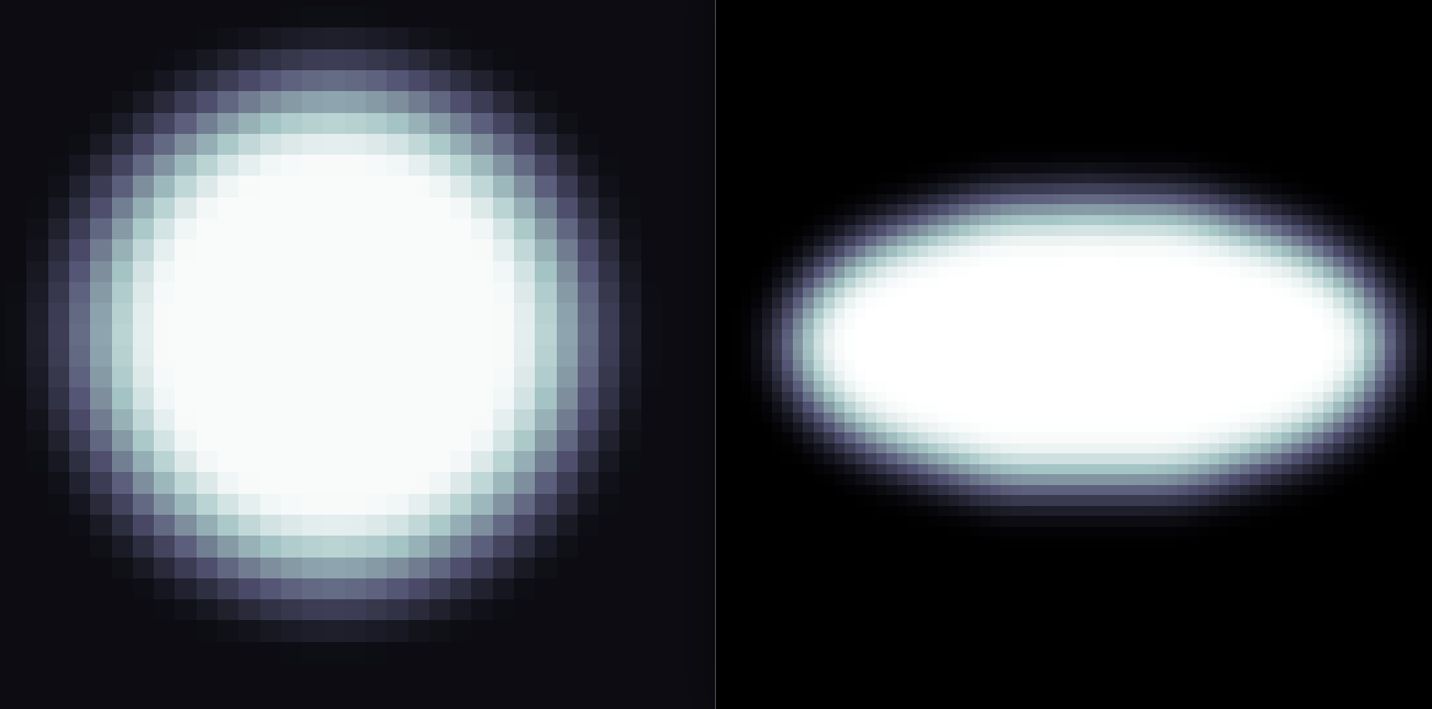
Logan Pearce found that convolving an elliptical-mask image with a circular 2D Tukey window will produce the desired elliptical 2D Tukey window.
Left: a circular Tukey window. Right: an elliptical Tukey window constructed by convolution.
sats
Coarsely determine the location of the star in pixels (i.e. just mouse over it). You can either shift to your
desired image center or record the pixel coordinate.
Subtract a radial profile from each image. Make sure the radial profile is centered under the star (~1 pixel
precision should be ok here).
Construct a mask of the same dimensions as for the unsats, but shifted to account for the position of the speckles
in the sats.
Construct a window with the same parameters as for the unsats, but shifted to account for the position of the speckles
in the sats.
Cross-Correlation
We can now use cross-correlation to register each of the sats to the reference image. Perform the following steps (order matters)
Apply the unsat-mask to the average RPS-unsat (the reference)
Normalize the result by subtracting the mean and dividing by the variance.
These operations should be performed only over the masked pixels (i.e. don’t include all the 0 pixels).
Note that this will create a discontinuity at the edge of the mask, necessitating windowing.
Apply the unsat-window to the result
Apply the sat-mask to one sat image
Normalize the result by subtracting the mean and dividing by the variance. These operations should be performed only over the masked pixels.
Apply the sat-window to the result
Cross-correlate the masked-normalized-windowed sat image with the masked-normalized-windowed unsat reference.
Record the shift.
To obtain sub-pixel precision you have several options:
Use the correlation theorem with small discrete FTs or with FFTs, and use a peak finding algorithm (e.g. Gaussian fit or center of light). This only kinda works.
Zero-pad the images before applying the correlation theorem. This is brutal. If you want 0.1 pixel resolution you need a 10:1 zero pad. Don’t even try.
Use a Matrix Fourier Transform. See this code for an example.
(note: the chi-squared error estimation available in that package does not seem to be useful for these purposes)
Repeat the last 4 steps for each sat image.
Error analysis
ToDo: describe bootstrap error analysis. The chi-squared map and Hessian techniques don’t work very well.